

mnist数据集
MNIST数据集是机器学习领域中非常经典的一个数据集,由60000个训练样本和10000个测试样本组成,每个样本都是一张28 * 28像素的灰度手写数字图片。
一共4个文件依次分别为:测试集、测试集标签、训练集、训练集标签

读入数据
使用TensorFlow中input_data.py脚本来读取数据及标签。
1 | from tensorflow.examples.tutorials.mnist import input_data |
数据可视化
将前20个图像显示出来。
1 | fig, ax = plt.subplots(nrows=4,ncols=5,sharex='all',sharey='all')#20个子图 |
图像如下

准备搭建卷积神经网络
本次采用3个卷积层和2个全连接层。
卷积函数和最大池化函数
1
2
3
4
5
6
7
8
9#定义卷积函数
def conv2d(x, w, b, k):
x = tf.nn.conv2d(x, w, strides=[1, k, k, 1], padding='SAME')
x = tf.add(x, b)
return tf.nn.relu(x)
#定义最大池化函数
def maxPool(x, k, s):
return tf.nn.max_pool(x, ksize=[1, k, k, 1], strides=[1, s, s, 1], padding='SAME')权值以及偏差
卷积核都是使用3*3。
1
2
3
4
5
6
7
8
9
10
11
12
13
14
15weights = {
'w1': tf.Variable(tf.random_normal([3, 3, 1, 32]), name='w1'),
'w2': tf.Variable(tf.random_normal([3, 3, 32, 64]), name='w2'),
'w3': tf.Variable(tf.random_normal([3, 3, 64, 128]), name='w3'),
'w4': tf.Variable(tf.random_normal([4*4*128, 625]), name='w4'),
'out': tf.Variable(tf.random_normal([625, 10]), name='wout')
}
biases = {
'b1': tf.Variable(tf.random_normal([32]), name='b1'),
'b2': tf.Variable(tf.random_normal([64]), name='b2'),
'b3': tf.Variable(tf.random_normal([128]), name='b3'),
'b4': tf.Variable(tf.random_normal([625]), name='b4'),
'out': tf.Variable(tf.random_normal([10]), name='bout')
}占位符
1
2
3
4
X = tf.placeholder(tf.float32, [None, 28, 28, 1], 'x')#输入
Y = tf.placeholder(tf.float32, [None, 10], 'y')#输出
p_conv = tf.placeholder(tf.float32, name='p_conv')#卷积层dropout的比例
p_hidden = tf.placeholder(tf.float32, name='p_hidden')#全连接层dropout的比例损失函数、优化器以及评估模型
1
2
3
4
5
6
7
# 损失函数
cost = tf.reduce_mean(tf.nn.softmax_cross_entropy_with_logits(logits=out, labels=Y))
#优化器
op = tf.train.AdamOptimizer(0.001).minimize(cost)
#评估模型
# argmax(array,axis) axis=1取每行最大值的索引,0为取每列最大值的索引。这里表示取每个样本的预测值
predict_op = tf.argmax(out, 1, name='predict_op')
搭建卷积神经网络
1 | def model(x, weight, biases, p_conv, p_hidden,): |
训练以及评估
因为数据量过大,所以采用分批训练。
1 | init = tf.global_variables_initializer() |
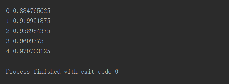
结果如下:
完整代码
1 | import tensorflow as tf |