1
2
3
4
5
6
7
8
9
10
11
12
13
14
15
16
17
18
19
20
21
22
23
24
25
26
27
28
29
30
31
32
33
34
35
36
37
38
39
40
41
42
43
44
45
46
47
48
49
50
51
52
53
54
55
56
57
58
59
60
61
62
63
64
65
66
67
68
69
70
71
72
73
74
75
76
77
78
79
80
81
| import tensorflow as tf
import numpy as np
import matplotlib.pyplot as plt
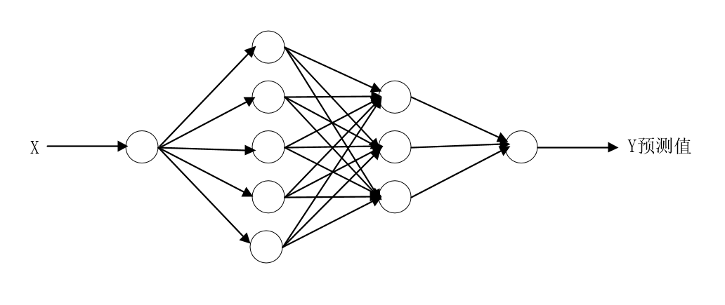
weights = {
'w1': tf.Variable(tf.random_normal([1, 5])),
'w2': tf.Variable(tf.random_normal([5, 3])),
'out': tf.Variable(tf.random_normal([3, 1]))
}
biases = {
'b1': tf.Variable(tf.random_normal([1, 5])),
'b2': tf.Variable(tf.random_normal([1, 3])),
'out': tf.Variable(tf.random_normal([1,1]))
}
learning_rate = 0.1
training_epochs = 1000
display_step = 100
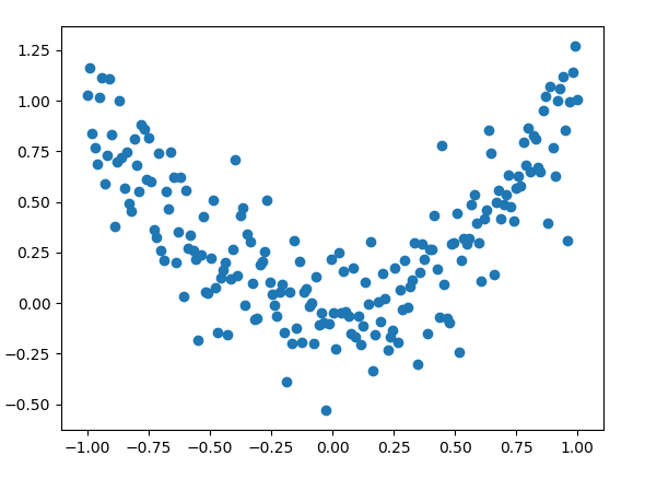
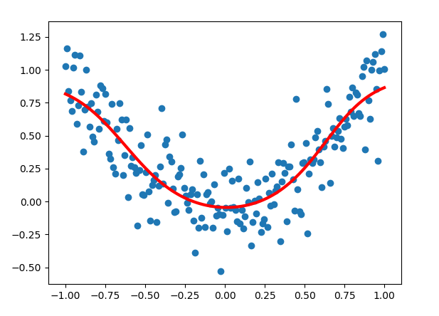
x_data=np.linspace(-1,1,200)[:, np.newaxis]
b=np.random.normal(0,0.2,x_data.shape)
y_data=np.square(x_data)+b
plt.scatter(x_data,y_data)
plt.show()
xs = tf.placeholder(tf.float32, [None, 1])
ys = tf.placeholder(tf.float32, [None, 1])
def network(x, weights, biases):
z1 = tf.add(tf.matmul(x, weights['w1']), biases['b1'])
a1 = tf.nn.tanh(z1)
z2 = tf.add(tf.matmul(a1, weights['w2']), biases['b2'])
a2 = tf.nn.tanh(z2)
z3 = tf.add(tf.matmul(a2, weights['out']), biases['out'])
outputs = tf.nn.tanh(z3)
return outputs
if __name__ == "__main__":
outputs = network(xs, weights, biases)
cost = tf.reduce_mean(tf.square(ys - outputs))
op = tf.train.GradientDescentOptimizer(learning_rate).minimize(cost)
init =tf.global_variables_initializer()
with tf.Session() as sess:
sess.run(init)
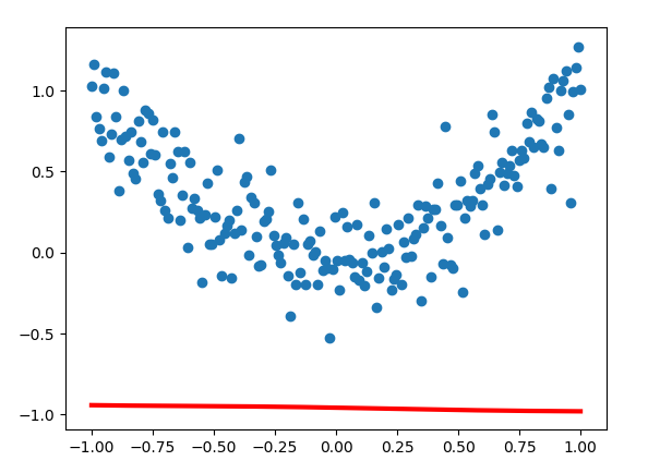
Y1 = sess.run(network(xs, weights, biases), feed_dict={xs: x_data, ys: y_data})
plt.scatter(x_data, y_data)
plt.plot(x_data, Y1, 'r-', lw=3)
plt.show()
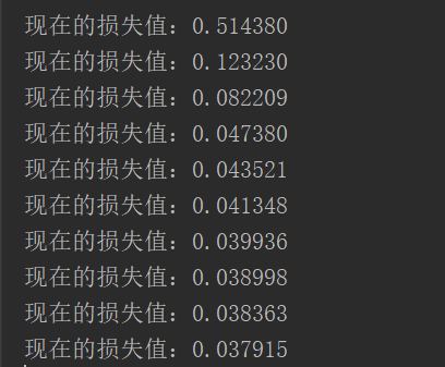
for i in range(training_epochs):
sess.run(op, feed_dict={xs: x_data, ys: y_data})
if i%display_step == 0:
print("现在的损失值:%f"%(sess.run(cost, feed_dict={xs: x_data, ys: y_data})))
Y = sess.run(network(xs, weights, biases), feed_dict={xs: x_data, ys: y_data})
plt.scatter(x_data,y_data)
plt.plot(x_data, Y, 'r-', lw=3)
plt.show()
|